Summer School Series: Lecture 3 by Vineet Gupta

This talk was delivered by Vineet Gupta , a research scientist at Google Brain, Mountain View California. His talk was titled Adaptive Optimization.

The optimization problem

The optimization problem aims to learn the best function from a class of functions. $$\operatorname{Class} : { \hat{y} = M(x | w), for \space w \in \mathbb{R}^{n} }\ $$

A class is most often specified as a neural network, parameterized by w. If the class is too large, overfitting happens. If the class is too small, well we end up getting bad results.

The most common function to find the best function is supervised learning.

Training examples: input output pairs such as (x₁, y₁),….(x_n, y_n)

Learning rule: Estimating $w$ such that $\hat{y_{i}} = M(x_{i}|w) \approx y_{i}$, and $w$ approximately minimizes $ F(w) = \sum_{i=1}^{n} l(\hat{y_{i}},y_{i})$ (the loss function)

In a feed-forward Deep Neural Network, gradient descent for the entire training is expensive. For this reason, we sample points and find the gradient for them.

Stochastic Optimization

The optimizer starts with the network denoted as $M(x|w)$.

At each round t: (the goal is to minimize $F(w)$)

• Optimizer has decided upon $w_{t}$
• Optimizer receives the input $ [x_{i} ]_{i=1}^{k}$
• Optimizer makes prediction $[\hat{y_{i}}= M(x_{i}|w_{t})]_{i=1}^{k}$
• Optimizer receives the true outcome
• Optimizer computes the loss $l_{t} = \sum_{i} l(y_{i},\hat{y_{i}})$ and gradient $g_{t} = \frac{\partial }{\partial w} \sum_{i} l(y_{i},\hat{y_{i}})$
• Optimizer uses $g_{t}$ to update $w_{t}$ to get $w_{t+1}$

We stop when the gradients vanish or run out of time (or epochs).

Regret

Convergence can be defined as the average loss compared to the optimum $w^{*}$

$$ R_{T} = \frac{1}{T} \sum_{t=1}^{T} l_{t} (w_{t}) - \frac{1}{T} \sum_{t=1}^{T} l_{t}(w^{*})$$

The proof of convergence can be picked up when $R_{T} \rightarrow 0 \text{ as } T \rightarrow 0$. This is a very strong requirement, regret tending to 0.

In convex optimization, $R_{T}$ can be computed in $O(\frac{1}{\sqrt{T}})$ time. Convex problems in SGD include faster convergence implies better condition number.

Momentum

What happens when the gradients become very noisy? To solve this, we can take a running average of the gradients. $$ \bar{g_{t}} = \gamma \bar{g_{t}} + (1-\gamma)g_{t}$$ Thus the momentum step becomes: $$w_{t+1} = w_{t}-\eta_{t} \bar{g_{t}}$$ The momentum approach works very well and is extremely popular, till date.

Another way to solve the problem is by using second order methods. To minimize $F(w)$,

$$F(w) \approx F(w_{t}) + (w - w_{t})^{T} \nabla F(w_{T}) + \frac{1}{2} (w - w_{t})^{T} \nabla^{2} F(w_{t}) (w - w_{t}) $$ (first two terms of the Taylor series).

The minimum is at: $w_{t+1} = w_{t} - \nabla^{2} F(w_{t})^{-1} \nabla F(w_{t})$

The biggest problem with this is computing the $\nabla^{2} F(w_{t})$ (Hessian) is very expensive, as it is a $n*n$ matrix with $n$ number of parameters.

AdaGrad

For gradient $g_{i}$ $$ H_{t} = \sqrt{(\sum_{s\leq{t}} g_{s} g_{s}^T)} $$

This is used as matrix for the Mahalnobis metric, that will be used. $$ \therefore w_{t+1} = \operatorname{argmin}_{w} \frac{1}{2\eta} ||w - w _{t}|| _{H _{t}}^{2} +\hat{l _{t}}(w) $$

The AdaGrad update rule is: $w_{t+1} = w_{t} - \eta H_{t}^{-1} g_{t}$. This is again very expensive, $O(n^{2})$ storage and $O(n^{3})$ time complexity per step.

The solution

One way to solve this is by the diagonal approximation, by taking only the diagonal matrix of the Hessian instead of the entire matrix. $$H_{t} = \operatorname{diag}{(\sum_{s\leq{t}}g_{s}g_{s}^{T}+\epsilon\operatorname{I})}^{\frac{1}{2}}$$

This take $O(n)$ space and $O(n)$ time per step.

AdaGrad has been so successful that there have been plenty of variants like AdaDelta/RMS Prop and Adam.

Full-matrix Preconditioning

AdaGrad Preconditioner

For $w_{t}$ of size 100 * 200, $g_{t}$ flattens to a 20,000 vector and then becomes 20k * 20k in size.

The Kronecker Product

Given a $m * n$ matrix $A$ and $p * q$ matrix $B$, their Kronecker Product $C$ is defined as $$C = A \bigotimes B $$ This is also called the matrix direct product, and is a $(mp)*(nq)$ matrix (every element of $A$ multiplied with $B$). It commutes with standard matrix product along with exponentials.

The Shampoo Preconditioner

The Shampoo Update:

Adagrad update: ${w} _{t+1} ={w} _{t}-\eta H _{t}^{-1} {g} _{t}$

Shampoo factorization: $w_{t+1}=w_{t}-\eta\left(L_{i}^{\frac{1}{4}} \otimes R_{t}^{\frac{1}{4}}\right)^{-1} g_{t}$

Shampoo update: $W_{t+1}=W_{t}-\eta L_{t}^{-\frac{1}{4}} G_{t} R_{t}^{-\frac{1}{4}}$ Theorem (convergence): If ${G} _{1}, \mathrm{G} _{2}, \ldots, \mathrm{G} _{\mathrm{T}}$ of rank $\leq \mathrm{r},$ then the rate of convergence is:

$$\frac{\sqrt{\mathrm{r}}}{\mathrm{T}} \operatorname{Tr}\left(\mathrm{L} _{\mathrm{T}}^{\frac{1}{4}}\right) \operatorname{Tr}\left(\mathrm{R} _{\mathrm{T}}^{\frac{1}{4}}\right)=\mathrm{O}\left(\frac{1}{\sqrt{\mathrm{T}}}\right)$$

$$({R_{t}}=\sum_{s \leq t} G_{s}^{\top} G_{s}$ and $L_{t}=\sum_{s \leq t} G_{s} G_{s}^{T})$$

Implementing Shampoo

The training system can be of two types:

• Asynchronous (accelerators don’t need to talk to each other, however it is hard for the parameter servers to handle)
• Synchronous (accelerator sends gradients to all the other accelerators, for them to average and update)

Challenges

• Tensorflow and PyTorch focus on 1^st order optimizations
• Computing $L_{t}^{-\frac{1}{4}}$ and $R_{t}^{-\frac{1}{4}}$ is expensive
• L, R have large condition numbers (upto the order of 10¹³).
• SVD is very expensive: $O(n^{3})$ in largest dimension
• Large layers are still impossible to precondition

Solutions

• Using high precision arithmetic (float 64), not performing the computations on a TPU.
• Computing preconditioners every 1000 steps is alright.
• Replace SVD with an iterative method
• Only matrix multiplications needed
  • Warm start: use previous preconditioner
  • Reduce condition number, remove top singular values
• Optimization for large layers
  • Precondition only one dimension
  • Block partioning the layer works better

Shampoo implementation and conclusion

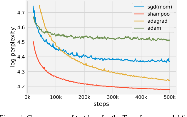
Shampoo gets implemented on a TPU+CPU. It is a little more expensive than AdaGrad but waay faster (saves 40% of the training time with 1.95 times fewer steps). Shampoo works well in language and speech domains, it isn’t suitable for image classication yet (for this Adam and AdaGrad work much better).

The Shampoo paper can be found here